STEP 5: Visualization
Visualization is essential for exploring ChIP-seq and ATAC-seq data. This page covers creating genome browser tracks and summary plots.
Creating BigWig Files
BigWig files allow visualization of coverage tracks in genome browsers like UCSC and IGV. They can be interpreted as continuous signal tracks showing read density across the genome.
Using bamCoverage (deepTools)
On the CCB:
module load deeptools
# OR
module load python-cbrg
Basic BigWig creation:
bamCoverage Parameters
-b- Input BAM file-o- Output bigWig file--binSize- Size of bins in bp (default 50) (can be set to 1 for highest resolution but larger file size)--normalizeUsing- Normalization method:RPKM- Reads Per Kilobase per Million mapped readsCPM- Counts Per Million (for non-length normalized)BPM- Bins Per MillionRPGC- Reads Per Genomic Content (requires genome size)
--smoothLength- Smooth signal over this many bp--numberOfProcessors- Number of threads
Increase --binSize and --smoothLength metrics for smoother data (less noisy), Decrease both to improve resolution, only better if sequencing is deeper
# For ATAC-seq (normalized and smoothed):
bamCoverage -b sample.mapped.sorted.rmdup.bam -o sample.smooth100.bs10.rpkm.bw \
    --binSize 10 \
    --smoothLength 100 \
    --normalizeUsing RPKM \
    --numberOfProcessors 8
Viewing in Genome Browsers
UCSC Genome Browser
To quickly visualize your bigWig files in the UCSC Genome Browser you need to move or copy them into the publically accessible folders (e.g. /project/higgslab/datashare/your_username/ on the CCB).
If a file test.bw is stored in /project/higgslab/datashare/your_username/Bigwigs the URL will be:
https://datashare.molbiol.ox.ac.uk/public/project/higgslab/your_username/Bigwigs/test.bwYou can use the loop to print the URL for multiple files:
cd /project/higgslab/datashare/your_username/Bigwigs

for file in *.bw; do
  echo "https://datashare.molbiol.ox.ac.uk/public/project/higgslab/your_username/Bigwigs/$file"
done
You can then copy all the URLs and add them as custom tracks in UCSC:
- Open UCSC Genome Browser
- Go to your reference genome (e.g., the same as you data such as mm39 for mouse)
- At the top of the page click on “My Data” -> “Custom Tracks”
- Paste in the URLS format for each bigWig file.
- Click “Submit” to add the tracks to your browser session.
- To change the display settings click on the track name and select “Configure Track”.
track name=test.bw description=Test bigDataUrl=https://datashare.molbiol.ox.ac.uk/public/project/higgslab/your_username/Bigwigs/test.bw type=bigWig color=0,0,255The color= parameter can be adjusted to change the RGB color of the track in UCSC using RGB values (0-255). Note this has to be “color” not “colour”. Also you can change the name= and description= fields to something more informative. Finally if you face errors, the most common have been due to incorrect URLs such as misordering of folders, or doubling /. The formats must be as listed in the type so make sure it’s a bigwig. Finally, files may have stringent permissions which maybe changed using chmod if you own the files.
This session can then be saved for future use by clicking on “My Data” -> “Sessions” -> “Save Session”. This is also useful for sharing with collaborators.
Creating Heatmaps with deepTools
DeepTools provides functions to create heatmaps and profile plots for visualizing signal enrichment around genomic features (e.g., TSS, peaks).
The deepTools suite has really usefult documentation: DeepTools Documentation
There are two main modes:
- reference-point: centered around a specific point (e.g., TSS, peak center)
- scale-regions: scales entire regions to a uniform length (e.g., gene bodies
Advanced examples
Heatmaps are only of biological interest when chosing the right regions to plot. For regions are provided in BED format. Please see Chapter 1.6 - BEDTools.
For the examples below, I used bedtools intersect to create a list of promoters that did not have CTCF binding in a 2kb window around the TSS, and then split these into active and inactive promoters based on H3K4me3 signal.
Plotting over scaled region with start and end points
### Plot Rad21 with scaled regions across all transcripts
computeMatrix scale-regions \
 -S mm10_Rad21_ChIP_WT_.rpkm.bw \           # Note that more than one signal file can be provided
 -R mm10_RefGene_transcripts_unique.bed \   # Note that more than one region file can be provided
 --binSize 20 \
 -o matrix_Rad21_mm10_scaledGenes.tab.gz \
 --beforeRegionStartLength 3000 \
 --regionBodyLength 5000 \
 --afterRegionStartLength 3000 \
 --skipZeros ;

plotHeatmap \
 -m matrix_Rad21_mm10_scaledGenes.tab.gz \
 -out Rad21_scaledGenes.png \
 --colorMap YlGnBu \                         # Note that if there are multiple signal files, multiple color maps can be provided
 --averageTypeSummaryPlot median \
 --regionsLabel 'genes' --samplesLabel 'Rad21 ChIP signal across scaled genes' \
 --heatmapHeight 15 \
 --sortRegions ascend \
 --legendLocation upper-right ;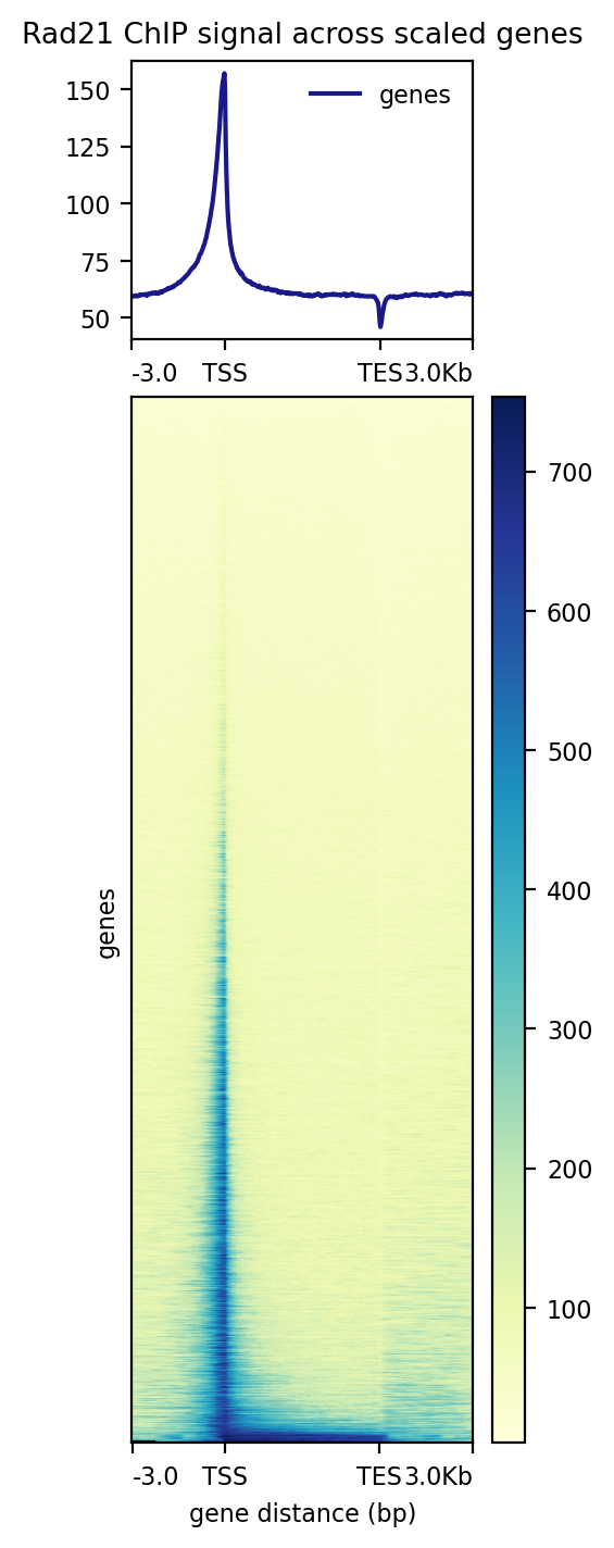
Plot Rad21 at in/active and non CTCF associated TSS
computeMatrix reference-point \
 -S mm10_Rad21_ChIP_WT.rpkm.bw \
 -R mm10_RefGene_transcripts_unique_no_CTCF_in_2kb_H3K4me3_inactive.TSS_2kb.bed mm10_RefGene_transcripts_unique_no_CTCF_in_2kb_H3K4me3_active.TSS_2kb.bed \
 --referencePoint center \
 -a 2000 -b 2000 \
 --binSize 20 \
 --skipZeros \
 -o matrix_Rad21_H3K4me3_active_vs_inactive_noCTCF_TSS.gz ;

plotHeatmap \
 -m matrix_Rad21_H3K4me3_active_vs_inactive_noCTCF_TSS.gz \
 -out Rad21_H3K4me3_active_vs_inactive_noCTCF_TSS.pdf \
 --averageTypeSummaryPlot median \
 --colorMap Blues \
 --heatmapHeight 15 \
 --samplesLabel 'Rad21 ChIP signal at TSS with no CTCF' \
 --regionsLabel 'inactive(n=14422)' 'active(n=8332)' \
 --refPointLabel 'TSS' \
 --sortRegions ascend \
 --legendLocation upper-right \
 --verbose ;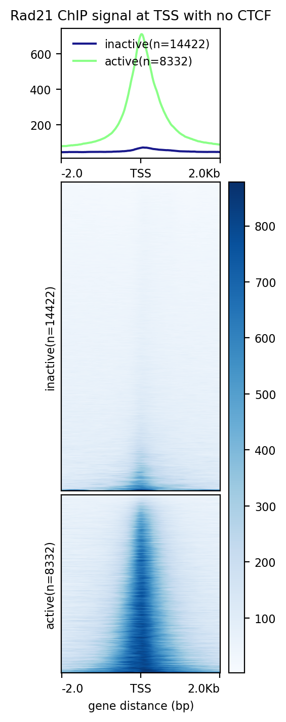
An example of how to run multple samples
# This is not a real path but is an example of how to use a variable for file paths
datashare_path="/project/higgslab/lcornell/Datashare/ChIPment_Data/"
#
computeMatrix scale-regions \
 -S "$datashare_path"CD71+/EB_CD71_PolII_WT_ChIPment.rpkm.bw \
 "$datashare_path"CD71+/151123_H3K4me3_notmESCs.smooth.rpkm.50.300.bw \
 "$datashare_path"CD71+/151123_H3K4me1_notmESCs.smooth.rpkm.50.300.bw \
 "$datashare_path"CD71+/LC_EB_CD71_E14_Input_ChIPment.rpkm.bw \
 -R mm39_refGene_unique_true.bed \
 -o Controls_Chipment_scaledGenes.tab.gz \
 --beforeRegionStartLength 3000 \
 --regionBodyLength 5000 \
 --afterRegionStartLength 3000 \
 --skipZeros ;

plotHeatmap \
 -m Controls_Chipment_scaledGenes.tab.gz \
 -out Controls_over_scaled_genes.png \
 --colorMap Oranges Greens BuGn Greys \
 --regionsLabel 'genes' \
 --samplesLabel 'PolII_CD71+' 'H3K4me3_CD71+' 'H3K4me1_CD71+' 'Input' \
 --zMin 0 0 0 0 --zMax 4 10 10 4 \
 --averageTypeSummaryPlot mean \
 --heatmapHeight 15 \
 --sortRegions ascend \
 --legendLocation upper-right ;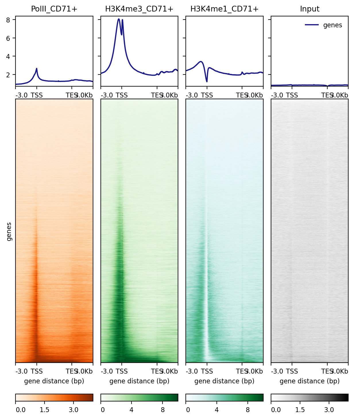
Creating IGV Snapshots
Use IGV’s batch scripting for automated snapshots:
new
genome mm39
load sample.bw
load peaks.bed
goto chr1:1000000-2000000
snapshot chr1_region.png
Next Steps
After visualization:
- Peak calling see STEP 6
- Quality assessments and Compareing replicates see STEP 7
- Identify differential regions and genomic features see STEP 8
- Generate publication-quality figures see PlotGardener