setwd("/Users/lucycornell/Documents/Higgs_post/Projects/18_BLP_2025_data/Caz_SNP_data/")STEP 7: Analysis Example Notebook
This notebook performs differential gene expression analysis between different conditions. In this example we have total RNA-seq from Ter119+ cells from mouse spleen which are WT or contain CTCF site deletions in the alpha globin locus: dt1, dt2, dt1t2. The count tables were created using featureCounts, on the .bams for each of the replicates:
featureCounts -t transcript -g gene_id \
 -a /project/higgslab/lcornell/BEDs/mm9.refGene.gtf \
 -p --countReadPairs \
 -s 0 -M -O --ignoreDup \
 -o All_CTCFdel_models_genes_featurecounts_table.txt \
 {all_the_input_.bams}
The output is a count table All_CTCFdel_models_genes_featurecounts_table.txt which is used for differential gene expression.
library(tidyverse)
library(matrixStats)
library(ggplot2)
library(DESeq2)
library(ashr)
library(reshape2)
library(dplyr)
### Read in data
exp=read.table("All_CTCFdel_models_genes_featurecounts_table.txt", sep='\t', header=T, check.names=FALSE)
colnames(exp) [1] "Geneid"
[2] "Chr"
[3] "Start"
[4] "End"
[5] "Strand"
[6] "Length"
[7] "D3theta_ter119/RNA_Dtheta2_ter119_rep1/RNA_Dtheta2_ter119_rep1.bam"
[8] "D3theta_ter119/RNA_Dtheta2_ter119_rep2/RNA_Dtheta2_ter119_rep2.bam"
[9] "D3theta_ter119/RNA_Dtheta2_ter119_rep3/RNA_Dtheta2_ter119_rep3.bam"
[10] "D53theta_ter119/RNA_Dt1t2_ter119_rep1/RNA_Dt1t2_ter119_rep1.bam"
[11] "D53theta_ter119/RNA_Dt1t2_ter119_rep2/RNA_Dt1t2_ter119_rep2.bam"
[12] "D53theta_ter119/RNA_Dt1t2_ter119_rep3/RNA_Dt1t2_ter119_rep3.bam"
[13] "D5theta_ter119/RNA_Dtheta1_ter119_rep1/RNA_Dtheta1_ter119_rep1.bam"
[14] "D5theta_ter119/RNA_Dtheta1_ter119_rep2/RNA_Dtheta1_ter119_rep2.bam"
[15] "D5theta_ter119/RNA_Dtheta1_ter119_rep3/RNA_Dtheta1_ter119_rep3.bam"
[16] "WT_ter119/RNA_WT_ter119_rep1/RNA_WT_ter119_rep1.bam"
[17] "WT_ter119/RNA_WT_ter119_rep2/RNA_WT_ter119_rep2.bam"
[18] "WT_ter119/RNA_WT_ter119_rep3/RNA_WT_ter119_rep3.bam" rownames(exp) = make.names(c(as.character(exp$Geneid)), unique=TRUE) # move the geneid names to the row ids
names(exp) = gsub("^.*/", "", names(exp))
names(exp) = gsub(pattern = ".bam", replacement = "", x = names(exp)) # removing ".bam" from column names
names(exp) = gsub(pattern = "RNA_", replacement = "", x = names(exp)) # removing "RNA" from column names
names(exp) = gsub(pattern = "_ter119", replacement = "", x = names(exp)) # removing "_ter119" from column names
colnames(exp) [1] "Geneid" "Chr" "Start" "End" "Strand"
[6] "Length" "Dtheta2_rep1" "Dtheta2_rep2" "Dtheta2_rep3" "Dt1t2_rep1"
[11] "Dt1t2_rep2" "Dt1t2_rep3" "Dtheta1_rep1" "Dtheta1_rep2" "Dtheta1_rep3"
[16] "WT_rep1" "WT_rep2" "WT_rep3" exp=exp[,c(7:ncol(exp))] # Keep only the count data
colnames(exp) [1] "Dtheta2_rep1" "Dtheta2_rep2" "Dtheta2_rep3" "Dt1t2_rep1" "Dt1t2_rep2"
[6] "Dt1t2_rep3" "Dtheta1_rep1" "Dtheta1_rep2" "Dtheta1_rep3" "WT_rep1"
[11] "WT_rep2" "WT_rep3" ## Set up comparison tables
exp.Condition=c(condition = c("Dtheta2","Dtheta2","Dtheta2",
"dt1t2","dt1t2","dt1t2",
"Dtheta1","Dtheta1","Dtheta1",
"WT","WT","WT"))
exp.SampleInfo=data.frame(condition=exp.Condition)
rownames(exp.SampleInfo)<-colnames(exp)
exp.SampleInfo condition
Dtheta2_rep1 Dtheta2
Dtheta2_rep2 Dtheta2
Dtheta2_rep3 Dtheta2
Dt1t2_rep1 dt1t2
Dt1t2_rep2 dt1t2
Dt1t2_rep3 dt1t2
Dtheta1_rep1 Dtheta1
Dtheta1_rep2 Dtheta1
Dtheta1_rep3 Dtheta1
WT_rep1 WT
WT_rep2 WT
WT_rep3 WT# Performing Differential expression analysis
exp.DESEQ2 <-DESeqDataSetFromMatrix(countData=exp,
colData=exp.SampleInfo,
design = ~ condition)# Make WT the primary comparison
colData(exp.DESEQ2)$condition <- relevel(colData(exp.DESEQ2)$condition, ref="WT")# Estimate size factors (library size normalization)
exp.DESEQ2 <- estimateSizeFactors(exp.DESEQ2)
# Check them
sizeFactors(exp.DESEQ2)Dtheta2_rep1 Dtheta2_rep2 Dtheta2_rep3 Dt1t2_rep1 Dt1t2_rep2 Dt1t2_rep3
0.9929277 1.3635304 1.8843127 0.8267914 0.7686396 1.6989033
Dtheta1_rep1 Dtheta1_rep2 Dtheta1_rep3 WT_rep1 WT_rep2 WT_rep3
0.5323157 1.1715425 1.0518824 0.7250312 0.7960567 1.1926184 exp.DESEQ2.analysis = DESeq(exp.DESEQ2)
res <- results(exp.DESEQ2.analysis)# transform counts (rlog or VST works better for PCA than raw counts)
vsd <- vst(exp.DESEQ2.analysis, blind=TRUE)
# or: vsd <- rlog(exp.DESEQ2.analysis, blind=TRUE)
# default PCA plot (built into DESeq2)
plotPCA(vsd, intgroup="condition") +
theme_classic()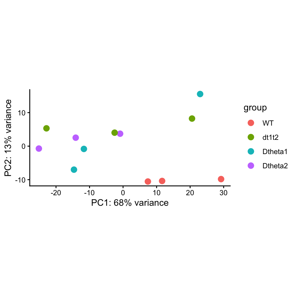
Running a single comparison and generating a MAplot with highlighted genes
This is contrasting dt1t2 to WT
res = results(exp.DESEQ2.analysis, contrast = c("condition", "dt1t2","WT"))

# performs moderation (shrinking) of log2 fold changes
res_lfc = lfcShrink(exp.DESEQ2.analysis,
                    coef="condition_dt1t2_vs_WT",
                    type="apeglm")

res$LFC = res_lfc$log2FoldChange

# Sort by adjusted p-value
res = res[order(res$padj), ]

res_df <- as.data.frame(res)

# Add coordinates as a column
res_df$geneid <- rownames(res_df)

# Reorder columns so coords is first
res_df <- res_df[, c("geneid", setdiff(names(res_df), "geneid"))]

# Filter for significant differences
sig_df <- subset(res_df, padj < 0.01)

# View first rows
head(sig_df)
geneid baseMean log2FoldChange lfcSE stat pvalue
Loxl2 Loxl2 25136.9981 11.678244 0.3965403 29.450331 1.246733e-190
Entpd4 Entpd4 3605.6533 6.630809 0.3883545 17.074114 2.313087e-65
Entpd4b Entpd4b 3603.7461 6.629989 0.3883522 17.072101 2.394264e-65
Hbq1b Hbq1b 180.4027 -3.404276 0.3514380 -9.686706 3.434256e-22
Snca Snca 29690.6735 13.121380 1.5677473 8.369576 5.782602e-17
Glrx Glrx 786.5058 2.914289 0.4007283 7.272481 3.529433e-13
padj LFC
Loxl2 1.637958e-186 11.647731
Entpd4 1.048528e-61 6.586497
Entpd4b 1.048528e-61 6.585703
Hbq1b 1.127981e-18 -3.328677
Snca 1.519436e-13 12.661931
Glrx 7.728282e-10 2.798291The MAplot generated also has highlights of genes that we are interested in (ie those in the Hba locus)
library(ggplot2)
library(ggrepel)

genes_of_interest <- c("Il9r", "Snrnp25", "Rhbdf1", "Mpg","Nprl3", "Hba.x",
                        "Hba.a1", "Sh3pxd2b","Ubtd2","Hbq1b", "Hbq1a")

# Build a plotting data frame from the DESeq2 results
plot_df <- as.data.frame(res_lfc)
plot_df$gene <- rownames(plot_df)
plot_df$log10baseMean <- log10(plot_df$baseMean + 1)

# Flag significance (treat NA padj as not significant)
plot_df$sig <- ifelse(!is.na(plot_df$padj) & plot_df$padj < 0.01, "padj < 0.01", "padj >= 0.01")

# Subset for genes of interest
goi_df <- plot_df[plot_df$gene %in% genes_of_interest, ]
goi_df$goi_col <- ifelse(!is.na(goi_df$padj) & goi_df$padj < 0.01, "padj < 0.01", "padj >= 0.01")

x_max <- max(plot_df$log10baseMean, na.rm = TRUE)

# MAplot
# Significant changes are in dark red and blue, non-significant changes are in grey or light red

ggplot(plot_df, aes(x = log10baseMean, y = log2FoldChange)) +
  geom_point(aes(color = sig), size = 1, alpha = 0.6) +
  scale_color_manual(values = c("padj < 0.01" = "blue", "padj >= 0.01" = "grey70")) +

  geom_point(data = goi_df,aes(x = log10baseMean, y = log2FoldChange, fill = goi_col),
             shape = 21, size = 3, stroke = 0) +
  scale_fill_manual(values = c("padj < 0.01" = "darkred", "padj >= 0.01" = "red")) +

  geom_text_repel(data = goi_df,
                   aes(x = log10baseMean, y = log2FoldChange, label = gene),
                   size = 3,
                   box.padding = 0.5,
                   point.padding = 0.3,
                   max.overlaps = Inf,
                   min.segment.length = 0) +
  coord_cartesian(xlim = c(0.5, x_max), ylim = c(-5, 5)) +
  labs(x = "Log10(Mean Normalised Counts + 1)",
       y = "Log2 Fold Change",
       title = "\u0394\u03B81\u03B82 vs WT", #This is how greek letters are printed in R!
       color = "All genes",
       fill = "Genes of interest") +
  theme_classic() +
  theme(plot.title = element_text(hjust = 0.5, face = "bold"),
        legend.position = "right")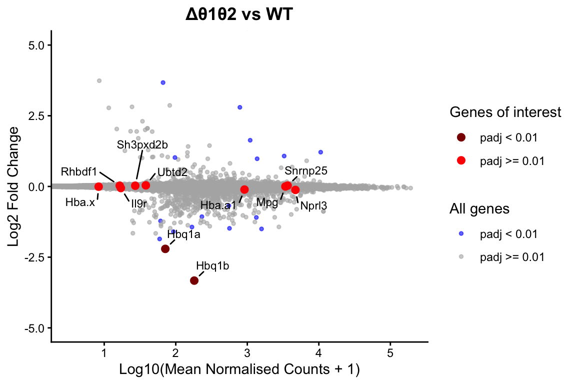
Generating analysis for multiple comparisons
### Compares each condition against WT reference, generating log2FoldChange with padj values

conditions <- c("Dtheta2", "dt1t2", "Dtheta1")
name <- "Total_RNAseq"

dir.create("ResultTables", showWarnings = FALSE)
dir.create("MAplots", showWarnings = FALSE)

# Containers to hold results for every condition, consistently named
res_list <- list()      # raw DESeq2 results (MLE log2FC)
res_lfc_list <- list()  # shrunken results (ashr)
res_df_list <- list()   # full results as data.frame, with normalized counts
sig_df_list <- list()   # subset of significant genes (padj < 0.01)

deseq_compare <- function(condition_name, ref = "WT", padj_cutoff = 0.01) {

  res <- results(exp.DESEQ2.analysis,
                  contrast = c("condition", condition_name, ref),
                  alpha = 0.05)

  res_lfc <- lfcShrink(exp.DESEQ2.analysis,
                        contrast = c("condition", condition_name, ref),
                        res = res,
                        type = "ashr")

  # Add shrunken LFC onto the raw results (keeps unshrunken log2FoldChange too)
  res$LFC <- res_lfc$log2FoldChange

  # Combine with normalized counts
  res_df <- cbind(as.data.frame(res),
                   as.data.frame(counts(exp.DESEQ2, normalized = TRUE)))
  res_df <- res_df[order(res_df$padj), ]
  res_df$geneid <- rownames(res_df)
  res_df <- res_df[, c("geneid", setdiff(names(res_df), "geneid"))]

  # Significant subset
  sig_df <- subset(res_df, padj < padj_cutoff)

  # Save results table
  write.csv(res_df,
            file = paste0("ResultTables/", name, ".Genes.", condition_name, "_vs_", ref, ".csv"),
            quote = FALSE, row.names = FALSE)

  # Save summary
  sink(file = paste0("ResultTables/", name, ".Summary.", condition_name, "_vs_", ref, ".txt"))
  print(summary(res, alpha = 0.05))
  sink()

  # Quick MA plot
  pdf(paste0("MAplots/", name, ".MAplot.", condition_name, "_vs_", ref, ".pdf"))
  plotMA(res_lfc, main = paste0(condition_name, " vs ", ref), ylim = c(-5, 5), alpha = 0.05)
  dev.off()

  # Return everything as a named list so results can be stored consistently
  list(res = res,
       res_lfc = res_lfc,
       res_df = res_df,
       sig_df = sig_df)
  }

# Run for all conditions and store results, keyed by condition name
all_results <- lapply(conditions, function(x) deseq_compare(x))
names(all_results) <- conditions
# Unpack into the separate lists (optional, if you prefer flat access)
for (cond in conditions) {
res_list[[cond]] <- all_results[[cond]]$res
res_lfc_list[[cond]] <- all_results[[cond]]$res_lfc
res_df_list[[cond]] <- all_results[[cond]]$res_df
sig_df_list[[cond]] <- all_results[[cond]]$sig_df
}
# Example access, consistent regardless of condition:
head(sig_df_list[["dt1t2"]]) geneid baseMean log2FoldChange lfcSE stat pvalue
Loxl2 Loxl2 25136.9981 11.678244 0.3965403 29.450331 1.246733e-190
Entpd4 Entpd4 3605.6533 6.630809 0.3883545 17.074114 2.313087e-65
Entpd4b Entpd4b 3603.7461 6.629989 0.3883522 17.072101 2.394264e-65
Hbq1b Hbq1b 180.4027 -3.404276 0.3514380 -9.686706 3.434256e-22
Snca Snca 29690.6735 13.121380 1.5677473 8.369576 5.782602e-17
Glrx Glrx 786.5058 2.914289 0.4007283 7.272481 3.529433e-13
padj LFC Dtheta2_rep1 Dtheta2_rep2 Dtheta2_rep3
Loxl2 1.583101e-186 11.635122 35155.6303 39017.8320 23763.0412
Entpd4 1.013412e-61 6.606376 6589.6035 3553.2761 1860.6254
Entpd4b 1.013412e-61 6.605558 6586.5821 3548.8758 1860.0947
Hbq1b 1.090205e-18 -3.339565 292.0656 266.9541 171.4153
Snca 1.468550e-13 12.402884 49995.5825 33946.4379 21565.4230
Glrx 7.469457e-10 2.785089 235.6667 178.2138 148.5953
Dt1t2_rep1 Dt1t2_rep2 Dt1t2_rep3 Dtheta1_rep1 Dtheta1_rep2
Loxl2 40271.34257 60120.508 33871.85079 28167.49418 19580.168679
Entpd4 6192.61395 7177.617 6256.38895 5047.75623 3421.984229
Entpd4b 6190.19496 7172.413 6252.85726 5045.87764 3421.984229
Hbq1b 25.39939 50.739 31.78521 67.62904 52.921682
Snca 49435.68551 65325.808 35552.34665 51351.10401 6.828604
Glrx 2206.11872 2909.036 2010.12026 381.35263 239.001143
Dtheta1_rep3 WT_rep1 WT_rep2 WT_rep3
Loxl2 21657.36337 6.896255 10.04954 21.800770
Entpd4 2969.91366 64.824793 67.83437 65.402311
Entpd4b 2968.01231 64.824793 67.83437 65.402311
Hbq1b 74.15277 496.530326 273.84985 361.389696
Snca 49091.98838 1.379251 11.30573 4.192456
Glrx 182.52991 531.011599 248.72601 167.698235Making boxplots of expression of individual genes
There may be times where you want to look directly at the changes of only a few genes. In this case we are interested in the expression of Hbq1b, which is the pseudogene near to the t1 CTCF site.
genes_of_interest <- c("Hbq1b","Hbq1a")

norm_counts <- counts(exp.DESEQ2.analysis, normalized=TRUE)
plot_df <- as.data.frame(norm_counts[genes_of_interest, , drop = FALSE])
plot_df$gene <- rownames(plot_df)
plot_df <- melt(plot_df, id.vars="gene", variable.name="sample", value.name="count")
plot_df$condition <- exp.SampleInfo$condition[match(plot_df$sample, rownames(exp.SampleInfo))]
plot_df$condition <- factor(plot_df$condition,
                            levels = c("WT", "Dtheta2","dt1t2","Dtheta1"))

# pull padj for genes of interest from the existing res_df_list ---
sig_df <- lapply(names(res_df_list), function(cond) {
  df <- res_df_list[[cond]]
  df <- df[df$geneid %in% genes_of_interest, c("geneid", "padj")]
  df$condition <- cond
  names(df)[names(df) == "geneid"] <- "gene"
  df
}) %>% bind_rows()

sig_df$condition <- factor(sig_df$condition, levels = c("WT","Dtheta2","dt1t2","Dtheta1"))

# Add sig labels for plotting
sig_df$label <- cut(sig_df$padj,
                    breaks=c(-Inf, 0.001, 0.01, 0.05, Inf),
                    labels=c("***", "**", "*", "ns"))

# y position per gene, scaled for free_y facets
y_pos <- plot_df %>%
  group_by(gene) %>%
  summarise(y = max(count, na.rm = TRUE) * 1.3)

sig_df <- left_join(sig_df, y_pos, by = "gene")

# Boxplots
ggplot(plot_df, aes(x=condition, y=count, color=condition)) +
  geom_jitter(width=0.15, size=2) +
  geom_boxplot(alpha=0.3, outlier.shape=NA) +
  scale_y_log10() +
  facet_wrap(~gene, scales="free_y") +
  theme_classic(base_size=14) +
  ylab("Normalized counts (log2)") +
  xlab("Condition") +
  ggtitle("Expression of selected genes") +
  geom_text(data = sig_df,
            aes(x = condition, y = y, label = label),
            inherit.aes = FALSE, size = 5, color = "black")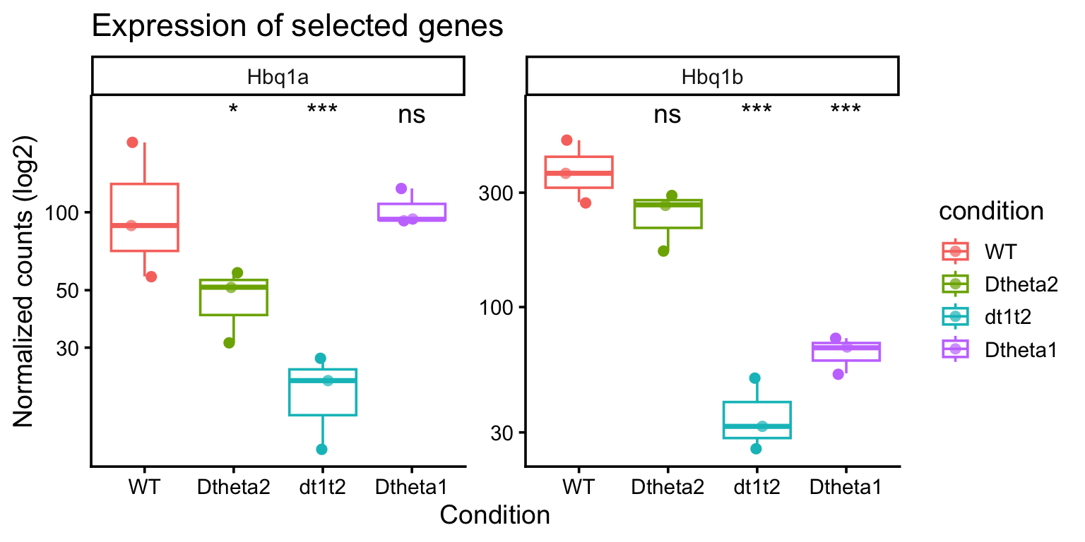
The Hbq1b gene is down regulated in the dt1t2 and dt1 models, which corresponds to the CTCF site deletion having an effect on expression. Equally for Hbq1a, there is a decrease in expression in the d2 and dt1t2 which again agrees with the deletion.
Exporting lists of up and down regulated genes
You may find that you want to intersect other differential regions of ChIP/ATAC signal with differential expression between conditions. You can define which genes are up, down or n.s. changed, then filter for these promoters as a bed file. You can then use something like bedtools intersect to compare with other regions of interest.
## Splitting TSS (+/- 1kb) based on Regulation in dt1t2 vs WT DESeq2 results

# Derive Regulation category: padj < 0.05 AND |log2FC| > 1
dt1t2_res <- res_df_list[["dt1t2"]]

dt1t2_res$Regulation <- "n.s."
dt1t2_res$Regulation[!is.na(dt1t2_res$padj) & dt1t2_res$padj < 0.05 & dt1t2_res$LFC > 1]  <- "up"
dt1t2_res$Regulation[!is.na(dt1t2_res$padj) & dt1t2_res$padj < 0.05 & dt1t2_res$LFC < -1] <- "down"

table(dt1t2_res$Regulation, useNA = "ifany")
 down  n.s.    up
    7 25195     7
# TSS bed file (mm9, matching featureCounts genome build)
tss = read.delim("mm9_RefGene_TSS_2x1000bp.bed", header = F)
names(tss) = c("chr", "start", "end", "refID", "score", "strand")
dir.create("TSSbeds", showWarnings = FALSE)
## UP
upreg = dt1t2_res[dt1t2_res$Regulation == "up",]
upreg.refID = upreg$geneid
tss.up = tss[tss$refID %in% upreg.refID,]
write.table(tss.up, "TSSbeds/mm9_RefGene_TSS_2x1000bp.dt1t2_vs_WT_UP.bed",
quote = F, col.names = F, row.names = F, sep = "\t")
## DOWN
downreg = dt1t2_res[dt1t2_res$Regulation == "down",]
downreg.refID = downreg$geneid
tss.down = tss[tss$refID %in% downreg.refID,]
write.table(tss.down, "TSSbeds/mm9_RefGene_TSS_2x1000bp.dt1t2_vs_WT_DOWN.bed",
quote = F, col.names = F, row.names = F, sep = "\t")
## N.s.
ns = dt1t2_res[dt1t2_res$Regulation == "n.s.",]
ns.refID = ns$geneid
tss.ns = tss[tss$refID %in% ns.refID,]
write.table(tss.ns, "TSSbeds/mm9_RefGene_TSS_2x1000bp.dt1t2_vs_WT_NonSign.bed",
quote = F, col.names = F, row.names = F, sep = "\t")
## Sanity check: row counts should roughly track table(dt1t2_res$Regulation) above
nrow(tss.up)[1] 7nrow(tss.down)[1] 7nrow(tss.ns)[1] 23112