Capture-C Analysis Example Notebook

This notebook analyses CaptureC counts from concatenated .gff files for a single viewpoint. It produces:

• Cis-normalised interaction profiles
• Smoothed plots with difference (subtraction) tracks
• Gene annotation tracks using plotgardener
• Significant contact changes between conditions using DESeq2

After running the CaptureC pipeline, each sample will have a concatenated .gff file per viewpoint with the following structure:

Chr	Analyser	Capture	Fragment start	Fragment End	Count	Strand	0	.
chr11	CC3	Hba-1	32179084	32179641	60	+	0	.
chr11	CC3	Hba-1	32179642	32179816	39	+	0	.

You can also download the .Rmd to run in RStudio on your own data: CaptureC Analysis Notebook

Loading the packages

library(tidyverse)
library(DESeq2)
library(cowplot)
library(zoo)
library(dplyr)

Define your gff inputs here

You can run this from concatenated .gffs per sample which have the column structure:

| chr  | source | viewpoint | reporter start | reporter end | count | strand | frame | attribute |
|------|--------|-----------|----------------|--------------|-------|--------|-------|-----------|
| chr1 | CC3    | Hba-1     | 10002466       | 10003091     | 1     | +      | 0     | .         |

files <- c(
  "Dt1t2_ter119_exp2_rep1_mm9_dpnii_concatenated.gff",
  "Dt1t2_ter119_exp2_rep2_mm9_dpnii_concatenated.gff",
  "Dt1t2_ter119_exp2_rep3_mm9_dpnii_concatenated.gff",
  "WT_ter119_exp2_rep1_mm9_dpnii_concatenated.gff",
  "WT_ter119_exp2_rep2_mm9_dpnii_concatenated.gff",
  "WT_ter119_exp2_rep3_mm9_dpnii_concatenated.gff"
)

# Remove the repetitive parts of the names 
# Change this according to your sample names

names <- basename(files)
names <- gsub("_ter119_exp2", "", names)
names <- gsub("_mm9_dpnii_concatenated\\.gff", "", names)

# Build a sample|condition table
sample_sheet <- data.frame(
  gff_file = files,
  filename = basename(files),
  sample = names,
  condition = gsub("_rep\\d+$", "", names),
  replicate = gsub(".*_(rep\\d+)$", "\\1", names))

sample_sheet

                                           gff_file
1 Dt1t2_ter119_exp2_rep1_mm9_dpnii_concatenated.gff
2 Dt1t2_ter119_exp2_rep2_mm9_dpnii_concatenated.gff
3 Dt1t2_ter119_exp2_rep3_mm9_dpnii_concatenated.gff
4    WT_ter119_exp2_rep1_mm9_dpnii_concatenated.gff
5    WT_ter119_exp2_rep2_mm9_dpnii_concatenated.gff
6    WT_ter119_exp2_rep3_mm9_dpnii_concatenated.gff
                                           filename     sample condition
1 Dt1t2_ter119_exp2_rep1_mm9_dpnii_concatenated.gff Dt1t2_rep1     Dt1t2
2 Dt1t2_ter119_exp2_rep2_mm9_dpnii_concatenated.gff Dt1t2_rep2     Dt1t2
3 Dt1t2_ter119_exp2_rep3_mm9_dpnii_concatenated.gff Dt1t2_rep3     Dt1t2
4    WT_ter119_exp2_rep1_mm9_dpnii_concatenated.gff    WT_rep1        WT
5    WT_ter119_exp2_rep2_mm9_dpnii_concatenated.gff    WT_rep2        WT
6    WT_ter119_exp2_rep3_mm9_dpnii_concatenated.gff    WT_rep3        WT
  replicate
1      rep1
2      rep2
3      rep3
4      rep1
5      rep2
6      rep3

# Define the control condition
ref_condition = "WT"

cond_levels <- unique(sample_sheet$condition)

# Reference first
cond_levels <- c(ref_condition, setdiff(cond_levels, ref_condition))

cond_string <- paste(cond_levels, collapse = "_vs_")

# Assign colours for the conditions

palette <- c("WT"="#262626", 
             "Dt1t2"="#1D91C0")

Define other inputs

# Choose your viewpoint to plot here
plot_viewpoint = "Hba-1"

# Path to the viewpoint coordinate file here
oligo_file = "Oligofile.txt"


# This loads it in
all_viewpoint = read_tsv(oligo_file, col_names = c("Viewpoint", "chr", "start", "end"))

viewpoint_coord = all_viewpoint[ all_viewpoint$Viewpoint == plot_viewpoint ,]

viewpoint_coord

# A tibble: 1 × 6
  Viewpoint   chr    start      end    X5 X6   
  <chr>     <dbl>    <dbl>    <dbl> <dbl> <chr>
1 Hba-1        11 32182969 32183821     1 A    

Define your plotting parameters

# Chromosome is imported from the viewpoint file 
chr_use = paste0("chr",viewpoint_coord$chr)

# Define the start and end coordinates of the whole plot
plot_start = 32020000
plot_end = 32300000
  
# Padding for the viewpoint exclusion 
excl_pad = 3000
excl_start = viewpoint_coord$start - excl_pad
excl_end = viewpoint_coord$end + excl_pad

# Padding for the viewpoint exclusion 
bin_size = 500
window_size_smooth = 2500

padj_thresh = 0.01

——— No editing is needed from here —————-

Loading the gff files

load_gff <- function(file, sample_name) {
  read_tsv(file, col_names = FALSE, comment = "#", show_col_types = FALSE) %>%
    transmute(
      capture = X3,
      chr = X1,
      start = as.numeric(X4),
      end = as.numeric(X5),
      count = as.numeric(X6),
      sample = sample_name,
      condition = strsplit(sample_name, "_")[[1]][1],
      midpoint = floor((start + end) / 2)
    )
}

all_df <- map2_df(sample_sheet$gff_file, sample_sheet$sample, load_gff) %>%
  filter(chr == chr_use) %>%
  filter(end < excl_start | start > excl_end)

if (nrow(all_df) == 0)
  stop("No fragments on ", chr_use, " — check chromosome naming in GFF files")

all_df

# A tibble: 65,065 × 8
   capture chr       start       end count sample     condition  midpoint
   <chr>   <chr>     <dbl>     <dbl> <dbl> <chr>      <chr>         <dbl>
 1 Hba-1   chr11 100142861 100143052     1 Dt1t2_rep1 Dt1t2     100142956
 2 Hba-1   chr11 100232583 100232994     1 Dt1t2_rep1 Dt1t2     100232788
 3 Hba-1   chr11 100392152 100392520     1 Dt1t2_rep1 Dt1t2     100392336
 4 Hba-1   chr11 100455808 100456194     1 Dt1t2_rep1 Dt1t2     100456001
 5 Hba-1   chr11 100537344 100537510     1 Dt1t2_rep1 Dt1t2     100537427
 6 Hba-1   chr11 100575601 100576546     1 Dt1t2_rep1 Dt1t2     100576073
 7 Hba-1   chr11 100611032 100611146     1 Dt1t2_rep1 Dt1t2     100611089
 8 Hba-1   chr11 100621841 100622623     3 Dt1t2_rep1 Dt1t2     100622232
 9 Hba-1   chr11 100666329 100667401     1 Dt1t2_rep1 Dt1t2     100666865
10 Hba-1   chr11 100669576 100669689     1 Dt1t2_rep1 Dt1t2     100669632
# ℹ 65,055 more rows

all_df %>%
  group_by(sample, capture) %>%
  summarise(n_fragments = n())

# A tibble: 30 × 3
# Groups:   sample [6]
   sample     capture  n_fragments
   <chr>      <chr>          <int>
 1 Dt1t2_rep1 Hba-1           6636
 2 Dt1t2_rep1 Hba-2           6659
 3 Dt1t2_rep1 Hbb-b1           385
 4 Dt1t2_rep1 Hbb-b2           405
 5 Dt1t2_rep1 Slc25A37         882
 6 Dt1t2_rep2 Hba-1           3188
 7 Dt1t2_rep2 Hba-2           3161
 8 Dt1t2_rep2 Hbb-b1           181
 9 Dt1t2_rep2 Hbb-b2           202
10 Dt1t2_rep2 Slc25A37         534
# ℹ 20 more rows

Filter for the viewpoint of interest

df = all_df[ all_df$capture == plot_viewpoint,]
df

# A tibble: 29,058 × 8
   capture chr       start       end count sample     condition  midpoint
   <chr>   <chr>     <dbl>     <dbl> <dbl> <chr>      <chr>         <dbl>
 1 Hba-1   chr11 100142861 100143052     1 Dt1t2_rep1 Dt1t2     100142956
 2 Hba-1   chr11 100232583 100232994     1 Dt1t2_rep1 Dt1t2     100232788
 3 Hba-1   chr11 100392152 100392520     1 Dt1t2_rep1 Dt1t2     100392336
 4 Hba-1   chr11 100455808 100456194     1 Dt1t2_rep1 Dt1t2     100456001
 5 Hba-1   chr11 100537344 100537510     1 Dt1t2_rep1 Dt1t2     100537427
 6 Hba-1   chr11 100575601 100576546     1 Dt1t2_rep1 Dt1t2     100576073
 7 Hba-1   chr11 100611032 100611146     1 Dt1t2_rep1 Dt1t2     100611089
 8 Hba-1   chr11 100621841 100622623     3 Dt1t2_rep1 Dt1t2     100622232
 9 Hba-1   chr11 100666329 100667401     1 Dt1t2_rep1 Dt1t2     100666865
10 Hba-1   chr11 100669576 100669689     1 Dt1t2_rep1 Dt1t2     100669632
# ℹ 29,048 more rows

df %>%
  group_by(sample, capture) %>%
  summarise(n_fragments = n())

# A tibble: 6 × 3
# Groups:   sample [6]
  sample     capture n_fragments
  <chr>      <chr>         <int>
1 Dt1t2_rep1 Hba-1          6636
2 Dt1t2_rep2 Hba-1          3188
3 Dt1t2_rep3 Hba-1          2932
4 WT_rep1    Hba-1          4281
5 WT_rep2    Hba-1          8520
6 WT_rep3    Hba-1          3501

Cis-Normalisation

Counts normalised to interactions per 100,000, cis-only, excluding the probe region.

norm_df <- df %>%
  group_by(sample) %>%
  mutate(norm_factor = sum(count)/100000,
         norm_count = count / norm_factor) %>%
  ungroup()

Difference tracks

Mean normalised count per condition with reference subtracted. Positive = more contacts; negative = fewer contacts than reference.

subtractions <- norm_df %>%
  group_by(chr, start, end, condition) %>%
  summarise(mean = mean(norm_count), .groups = "drop") %>%
  pivot_wider(names_from = condition, values_from = mean, values_fill = 0) %>%
  
  mutate(across(all_of(setdiff(cond_levels, ref_condition)),
                ~ .x - .data[[ref_condition]],
                .names = "{.col}_minus_{ref_condition}")) %>%
  
  filter(start >= plot_start, end <= plot_end)

subtractions

# A tibble: 602 × 6
   chr      start      end    WT Dt1t2 Dt1t2_minus_WT
   <chr>    <dbl>    <dbl> <dbl> <dbl>          <dbl>
 1 chr11 32020271 32021268 10.4   7.11         -3.27 
 2 chr11 32021294 32023427 15.6  17.9           2.29 
 3 chr11 32023428 32024368  7.08  6.26         -0.822
 4 chr11 32024369 32026059  6.39  8.95          2.57 
 5 chr11 32026060 32026215  0     7.11          7.11 
 6 chr11 32026216 32026512  7.81  8.43          0.620
 7 chr11 32026513 32026549 18.0   0           -18.0  
 8 chr11 32026550 32026817  3.54  0            -3.54 
 9 chr11 32026818 32027130  7.08  3.56         -3.52 
10 chr11 32027131 32027802  9.01 12.9           3.90 
# ℹ 592 more rows

Bin and smooth

500 bp bins, 2500 bp sliding window. Each replicate smoothed individually before averaging across replicates.

# Bins
bins <- tibble(
  bin_start = seq(plot_start, plot_end - bin_size, by = bin_size)) %>%
  mutate(bin_end = bin_start + bin_size - 1, bin_id = row_number())

windowbins <- floor(((window_size_smooth / bin_size) - 1) / 2)
bins_contributing <- 2 * windowbins + 1

# Bin, smooth per replicate, then summarise per condition
summary_df <- norm_df %>%
  cross_join(bins) %>%
  filter(end > bin_start, start < bin_end) %>%
  mutate(overlap_bp = pmax(0, pmin(end, bin_end) - pmax(start, bin_start)),
         weighted_count = norm_count * (overlap_bp / bin_size)) %>%
  
  group_by(chr, bin_id, bin_start, bin_end, sample, condition) %>%
  summarise(binned_count = sum(weighted_count), .groups = "drop") %>%
  arrange(condition, sample, bin_start) %>%
  group_by(condition, sample) %>%
  mutate(smoothed_count = rollmean(binned_count, k = bins_contributing,
                              align = "center", fill = "extend"),
          pos = bin_start + (bin_end - bin_start) / 2) %>%
  ungroup() %>%
  group_by(pos, condition) %>%
  summarise(mean_count = mean(smoothed_count),
            sd_count = sd(smoothed_count),
            .groups = "drop")

summary_df

# A tibble: 1,076 × 4
         pos condition mean_count sd_count
       <dbl> <chr>          <dbl>    <dbl>
 1 32020250. Dt1t2           4.41   NA    
 2 32020250. WT              9.95    2.93 
 3 32020750. Dt1t2           4.41   NA    
 4 32020750. WT              8.31    0.961
 5 32021250. Dt1t2           9.96    7.84 
 6 32021250. WT              9.95    2.93 
 7 32021750. Dt1t2          15.5    NA    
 8 32021750. WT             12.1     1.57 
 9 32022250. Dt1t2          15.5    NA    
10 32022250. WT             13.7     2.39 
# ℹ 1,066 more rows

Build exclusion zones for plotting

all_viewpoint

# A tibble: 5 × 6
  Viewpoint   chr     start       end    X5 X6   
  <chr>     <dbl>     <dbl>     <dbl> <dbl> <chr>
1 Hba-1        11  32182969  32183821     1 A    
2 Hba-2        11  32195804  32196638     1 A    
3 Hbb-b1        7 110961967 110962817     1 A    
4 Hbb-b2        7 110975976 110976456     1 A    
5 Slc25A37     14  69902454  69903469     1 A    

viewpoint_start = viewpoint_coord$start
viewpoint_end = viewpoint_coord$end

# Globin duplicate: separate exclusion zone for the partner probe
partner_excl <- NULL

globin_pairs <- list(
  c("Hba-1", "Hba-2"),
  c("Hba-a1", "Hba-a2"),
  c("Hbb-b1", "Hbb-b2"))

partner_vp <- NULL
for (pair in globin_pairs) {
  if (plot_viewpoint %in% pair) {
    partner_vp <- setdiff(pair, plot_viewpoint)
    break
  }
}

if (!is.null(partner_vp) && length(partner_vp) == 1) {
  partner_coord <- all_viewpoint[all_viewpoint$Viewpoint == partner_vp, ]
  if (nrow(partner_coord) == 0) {
    message("Partner viewpoint '", partner_vp,
            "' not found in oligo file — skipping partner exclusion zone")
    partner_excl <- NULL
  } else {
    partner_excl <- list(
      start = partner_coord$start[1] - excl_pad,
      end = partner_coord$end[1]   + excl_pad,
      probe_start = partner_coord$start[1],
      probe_end = partner_coord$end[1]
    )
    message("Globin duplicate: adding exclusion zone for ", partner_vp)
  }
} else {
  partner_excl <- NULL
}

add_annotations <- function(p) {
  p <- p +
    # Primary viewpoint exclusion zone
    geom_rect(aes(xmin = excl_start, xmax = excl_end, ymin = -Inf, ymax = Inf),
              inherit.aes = FALSE, fill = "white", color = "black") +
    # Primary viewpoint probe
    geom_rect(aes(xmin = viewpoint_start, xmax = viewpoint_end, ymin = -Inf, ymax = Inf),
              inherit.aes = FALSE, fill = "black")

  # Partner probe exclusion zone (globin duplicates only)
  if (!is.null(partner_excl)) {
    p <- p +
      geom_rect(aes(xmin = partner_excl$start, xmax = partner_excl$end, ymin = -Inf, ymax = Inf),
                inherit.aes = FALSE, fill = "white", color = "black") +
      geom_rect(aes(xmin = partner_excl$probe_start, xmax = partner_excl$probe_end, ymin = -Inf, ymax = Inf),
                inherit.aes = FALSE, fill = "black")
  }
  p
}

Main plot

p1 <- ggplot(summary_df, aes(x = pos, y = mean_count, color = condition, fill = condition)) +
  geom_ribbon(aes(ymin = mean_count - sd_count, 
                  ymax = mean_count + sd_count),
              alpha = 0.15, color = NA) +
  geom_line(linewidth = 0.6, alpha = 0.9) +
  scale_color_manual(values = palette) +
  scale_fill_manual(values = palette) +
  scale_x_continuous(limits = c(plot_start, plot_end), expand = c(0, 0)) +
  scale_y_continuous(expand = c(0, 0)) +
  labs(y = "Mean interactions per fragment",
       x = paste0(chr_use, " position (bp)"),
       color = NULL, fill = NULL,
       title = paste0(plot_viewpoint, "  |  ", chr_use, ":",
                      format(plot_start, big.mark = ","), " – ",
                      format(plot_end, big.mark = ","))) +
  theme_bw() +
  theme(panel.grid = element_blank(),
        legend.position = c(0.98, 0.5), 
        legend.justification = c("right", "center"),
        legend.direction = "vertical", 
        text = element_text(size = 12)) 

p1 <- add_annotations(p1)
p1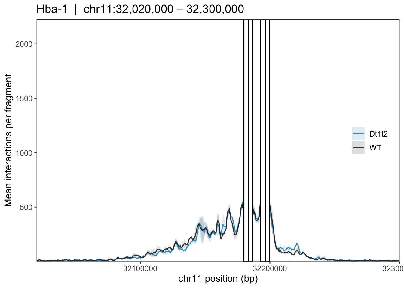

Subtraction plots

delta_plot_list <- map(setdiff(cond_levels, ref_condition), function(cond) {
  delta_col <- paste0(cond, "_minus_", ref_condition)
  y_lim <- max(abs(range(subtractions[[delta_col]], na.rm = TRUE))) * 1.1
  
  p <- ggplot(subtractions) +
    geom_rect(aes(xmin = start, xmax = end, ymin = 0, ymax = .data[[delta_col]]),
              fill = palette[[cond]], alpha = 0.75) +
    geom_hline(yintercept = 0, linewidth = 0.3, color = "grey40") +
    scale_x_continuous(limits = c(plot_start, plot_end), expand = c(0, 0)) +
    scale_y_continuous(limits = c(-y_lim, y_lim), expand = c(0, 0),
                       breaks = pretty(c(-y_lim, y_lim), n = 3)) +
    labs(y = bquote(Delta ~ .(cond) - .(ref_condition)),
         x = paste0(chr_use, " position (bp)")) +
    theme_bw() +
    theme(panel.grid = element_blank(),
          text = element_text(size = 12))
  
  add_annotations(p)
})

Combined plots

# Remove x axis from main plot
p1 <- p1 + theme(axis.title.x = element_blank(),
                 axis.text.x = element_blank(),
                 axis.ticks.x = element_blank())

# Remove x axis from all delta plots except the last
n <- length(delta_plot_list)
delta_plot_list[-n] <- map(delta_plot_list[-n], ~ .x +
    theme(axis.title.x = element_blank(),
          axis.text.x = element_blank(),
          axis.ticks.x = element_blank()))

all_plots <- c(list(p1), delta_plot_list)

rel_heights <- c(2.5, rep(1, length(delta_plot_list)))

final_plot <- plot_grid(plotlist = all_plots, ncol = 1,
                        align = "v", axis = "l", rel_heights = rel_heights)

final_plot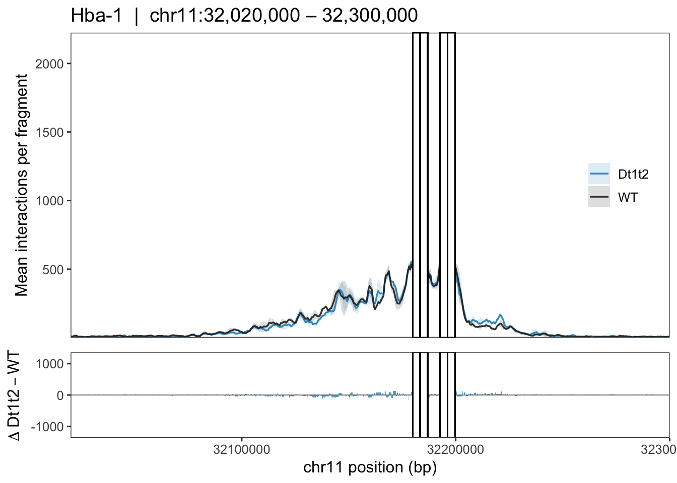

# ggsave(plot_file, plot = final_plot, width = 10, height = 4 + 2 * length(delta_plot_list), units = "in")

Combining with gene annotations

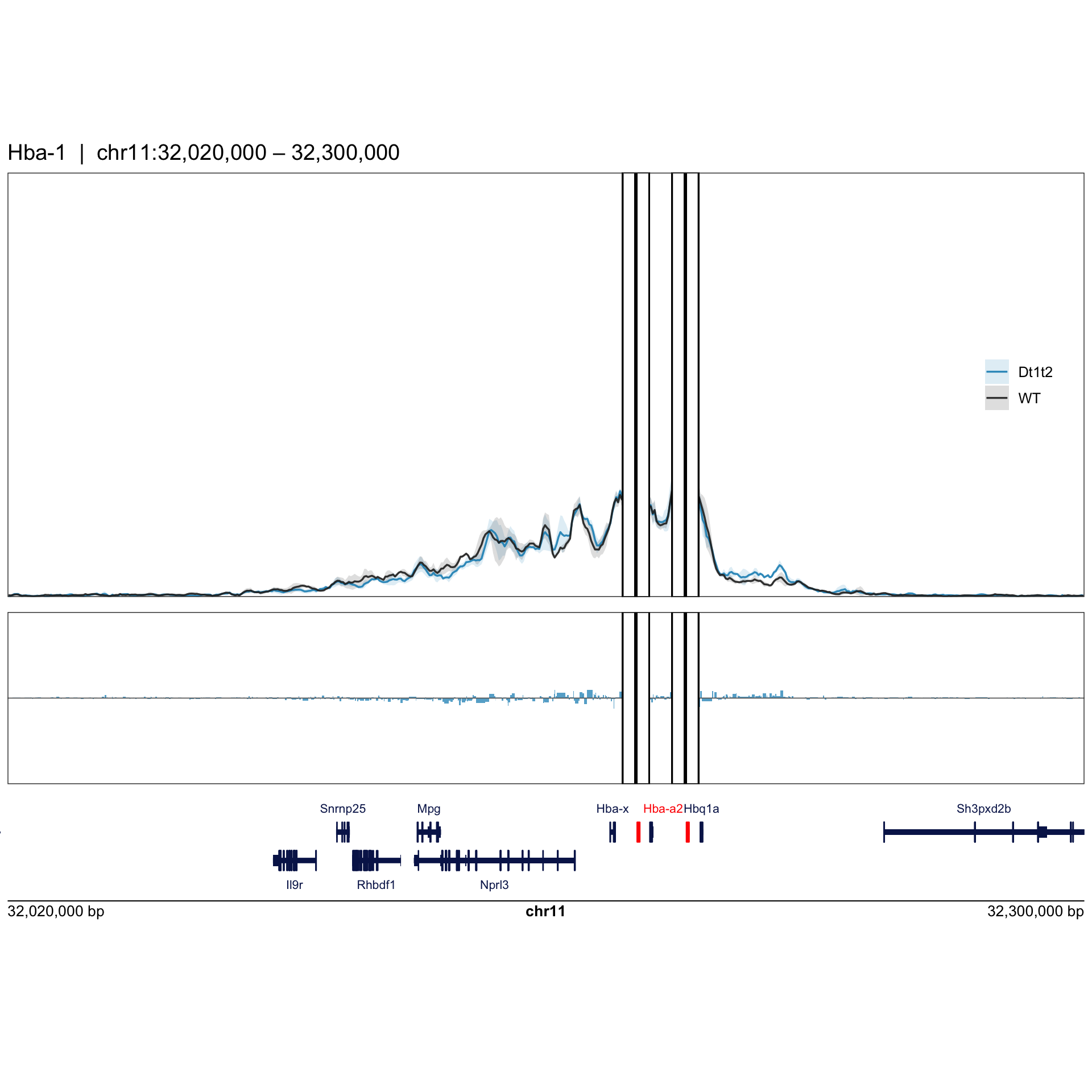
First we have to strip the axis text from all plots so the panel starts at a known, fixed x position — this is what lets plotgardener align underneath

p1 <- p1 +
  theme(axis.title.x = element_blank(),
        axis.text.x = element_blank(),
        axis.ticks.x = element_blank(),
        axis.title.y = element_blank(),
        axis.text.y = element_blank(),
        axis.ticks.y = element_blank(),
        plot.margin = margin(t = 5, r = 5, b = 5, l = 5, unit = "pt"))

delta_plot_list <- map(delta_plot_list, ~ .x +
  theme(axis.title.x = element_blank(),
        axis.text.x  = element_blank(),
        axis.ticks.x = element_blank(),
        axis.title.y = element_blank(),
        axis.text.y  = element_blank(),
        axis.ticks.y = element_blank(),
        plot.margin  = margin(t = 5, r = 5, b = 5, l = 5, unit = "pt")))

# Rebuild the combined plot with the stripped axes
all_plots <- c(list(p1), delta_plot_list)
rel_heights <- c(2.5, rep(1, length(delta_plot_list)))

final_plot <- plot_grid(plotlist = all_plots, ncol = 1,
                        align = "v", axis = "l", rel_heights = rel_heights)

Then adding in the gene annotations using plotgardener. Make sure to change the library called here and genome assembly to add the correct annotations.

library(plotgardener)

# Make sure to load/download the correct genome for your analysis
library(TxDb.Mmusculus.UCSC.mm9.knownGene)
library(org.Mm.eg.db)

gene_track_height <- 1
existing_height <- 4 + 2 * length(delta_plot_list)
total_height <- existing_height + gene_track_height

# Fixed margin in inches (5pt plot.margin ≈ 0.07in) — same for ggplot panel and gene track
track_x <- 0.07
track_width <- 10 - (2 * track_x)

{
  pageCreate(width = 10, height = total_height + 0.5, default.units = "inches",
             showGuides = FALSE)
  
  ## Genomic and dimension parameters
  params_c <- pgParams(chrom = chr_use, chromstart = plot_start, chromend = plot_end,
                       assembly = "mm9", x = track_x, width = track_width,
                       default.units = "inches")
  
  # --- Combined ggplot at the top ---
  plotGG(plot = final_plot, x = 0, y = 0,
         width = 10, height = existing_height,
         just = c("left", "top"))
  
  # --- Gene annotation track ---
  genes <- plotGenes(params = params_c, stroke = 0.05, fontsize = 8, 
                     geneHighlights = data.frame("gene" = c("Hba-a1","Hba-a2"),"color" = c("red", "red")),
                     geneBackground = "#081D58", strandLabels = TRUE,
                     y = existing_height, height = gene_track_height)
  
  # --- Genomic coordinate ruler ---
  annoGenomeLabel(params = params_c, plot = genes, y = existing_height + gene_track_height)
}

DESeq2 statistical testing

DESeq2 uses raw (un-normalised) counts. Tests each fragment for significant contact differences between conditions.

Column	Meaning
baseMean	Average normalised count across all samples
log2FoldChange	log₂(test / reference) — positive = more contacts in test
padj	Adjusted p-value — use this for significance
direction	up = gain, down = loss of contacts vs reference

# Raw count matrix from df (no excl filter — we want all fragments for DESeq2)
count_mat <- df %>%
  mutate(fragment = paste0(chr, ":", start, "-", end)) %>%
  dplyr::select(fragment, sample, count) %>%
  dplyr::distinct() %>%
  pivot_wider(names_from = sample,
              values_from = count,
              values_fill = 0)

counts <- as.matrix(count_mat[, -1])
rownames(counts) <- count_mat$fragment

# Build the sample sheet for comparisons
coldata <- data.frame(row.names = sample_sheet$sample,
                      condition = factor(sample_sheet$condition, levels = cond_levels))

dds <- DESeqDataSetFromMatrix(countData = counts,
                              colData = coldata,
                              design = ~condition)

# Run DESeq
dds <- DESeq(dds)

# Extract the results, comparing reference to each condition  

get_results <- function(test_cond, ref_cond) {
  as.data.frame(results(dds, contrast = c("condition", test_cond, ref_cond))) %>%
    rownames_to_column("fragment") %>%
    separate(fragment, into = c("chr", "coords"), sep = ":",  extra = "merge") %>%
    separate(coords, into = c("start", "end"),  sep = "-",  convert = TRUE) %>%
    mutate(comparison = paste0(test_cond, "_vs_", ref_cond),
           direction = case_when(is.na(padj) ~ NA_character_,
                                 log2FoldChange > 0 ~ "up",
                                 log2FoldChange < 0 ~ "down",
                                 TRUE ~ "unchanged"),
           chr = as.character(chr),
           start = as.integer(start),
           end = as.integer(end)) %>%
    dplyr::select(comparison, chr, start, end,
           baseMean, log2FoldChange, lfcSE, stat, pvalue, padj, direction)
}

non_ref <- setdiff(cond_levels, ref_condition)

all_results <- map(non_ref, ~ get_results(.x, ref_condition)) %>%
  bind_rows()

sig_results <- all_results %>%
  filter(!is.na(padj), padj < padj_thresh) %>%
  arrange(padj)

print(paste0("Number of significant differences for ", plot_viewpoint ,":  ", nrow(sig_results)))

[1] "Number of significant differences for Hba-1:  0"

# Write outputs to tables

all_out <- file.path(paste0(plot_viewpoint, "_", cond_string, "_DESeq2_all_results.tsv"))
write_tsv(all_results, all_out)

sig_out <- file.path(paste0(plot_viewpoint, "_", cond_string, "_DESeq2_significant.tsv"))
write_tsv(sig_results, sig_out)

sessionInfo()

R version 4.5.1 (2025-06-13)
Platform: x86_64-apple-darwin20
Running under: macOS Tahoe 26.5.1

Matrix products: default
BLAS:   /Library/Frameworks/R.framework/Versions/4.5-x86_64/Resources/lib/libRblas.0.dylib 
LAPACK: /Library/Frameworks/R.framework/Versions/4.5-x86_64/Resources/lib/libRlapack.dylib;  LAPACK version 3.12.1

locale:
[1] C.UTF-8/C.UTF-8/C.UTF-8/C/C.UTF-8/C.UTF-8

time zone: Europe/London
tzcode source: internal

attached base packages:
[1] stats4    stats     graphics  grDevices utils     datasets  methods  
[8] base     

other attached packages:
 [1] org.Mm.eg.db_3.21.0                    
 [2] TxDb.Mmusculus.UCSC.mm9.knownGene_3.2.2
 [3] GenomicFeatures_1.60.0                 
 [4] AnnotationDbi_1.70.0                   
 [5] plotgardener_1.14.0                    
 [6] zoo_1.8-15                             
 [7] cowplot_1.2.0                          
 [8] DESeq2_1.48.2                          
 [9] SummarizedExperiment_1.38.1            
[10] Biobase_2.68.0                         
[11] MatrixGenerics_1.20.0                  
[12] matrixStats_1.5.0                      
[13] GenomicRanges_1.60.0                   
[14] GenomeInfoDb_1.44.3                    
[15] IRanges_2.42.0                         
[16] S4Vectors_0.46.0                       
[17] BiocGenerics_0.54.1                    
[18] generics_0.1.4                         
[19] lubridate_1.9.5                        
[20] forcats_1.0.1                          
[21] stringr_1.6.0                          
[22] dplyr_1.2.1                            
[23] purrr_1.2.2                            
[24] readr_2.2.0                            
[25] tidyr_1.3.2                            
[26] tibble_3.3.1                           
[27] ggplot2_4.0.3                          
[28] tidyverse_2.0.0                        

loaded via a namespace (and not attached):
 [1] DBI_1.3.0                bitops_1.0-9             rlang_1.2.0             
 [4] magrittr_2.0.5           otel_0.2.0               RSQLite_3.52.0          
 [7] compiler_4.5.1           png_0.1-9                vctrs_0.7.3             
[10] pkgconfig_2.0.3          crayon_1.5.3             fastmap_1.2.0           
[13] XVector_0.48.0           labeling_0.4.3           utf8_1.2.6              
[16] Rsamtools_2.24.1         rmarkdown_2.31           tzdb_0.5.0              
[19] UCSC.utils_1.4.0         strawr_0.0.92            bit_4.6.0               
[22] xfun_0.57                cachem_1.1.0             jsonlite_2.0.0          
[25] blob_1.3.0               rhdf5filters_1.20.0      DelayedArray_0.34.1     
[28] Rhdf5lib_1.30.0          BiocParallel_1.42.2      parallel_4.5.1          
[31] R6_2.6.1                 plyranges_1.28.0         stringi_1.8.7           
[34] RColorBrewer_1.1-3       rtracklayer_1.68.0       Rcpp_1.1.1-1.1          
[37] knitr_1.51               Matrix_1.7-5             timechange_0.4.0        
[40] tidyselect_1.2.1         dichromat_2.0-0.1        abind_1.4-8             
[43] yaml_2.3.12              codetools_0.2-20         curl_7.1.0              
[46] lattice_0.22-9           KEGGREST_1.48.1          withr_3.0.2             
[49] S7_0.2.2                 evaluate_1.0.5           gridGraphics_0.5-1      
[52] Biostrings_2.76.0        pillar_1.11.1            vroom_1.7.1             
[55] RCurl_1.98-1.18          hms_1.1.4                scales_1.4.0            
[58] glue_1.8.1               tools_4.5.1              BiocIO_1.18.0           
[61] data.table_1.18.4        locfit_1.5-9.12          GenomicAlignments_1.44.0
[64] fs_2.1.0                 XML_3.99-0.23            rhdf5_2.52.1            
[67] grid_4.5.1               GenomeInfoDbData_1.2.14  restfulr_0.0.16         
[70] cli_3.6.6                rappdirs_0.3.4           S4Arrays_1.8.1          
[73] gtable_0.3.6             yulab.utils_0.2.4        digest_0.6.39           
[76] SparseArray_1.8.1        ggplotify_0.1.3          rjson_0.2.23            
[79] htmlwidgets_1.6.4        farver_2.1.2             memoise_2.0.1           
[82] htmltools_0.5.9          lifecycle_1.0.5          httr_1.4.8              
[85] bit64_4.8.0             

This notebook also plots the genes under the plot and you have a bit more freedom to change the asthetics.